Reporting and adjusting PGS in the context of genetic ancestry

v2 of the pgsc_calc pipeline introduces the ability to analyse the genetic ancestry of the individuals in your sampleset in comparison to a reference panel (default: 1000 Genomes) using principal component analysis (PCA). In this document we explain how the PCA is derived, and how it can be used to report polygenic scores that are adjusted or contextualized by genetic ancestry using multiple different methods.

Motivation: PGS distributions and genetic ancestry

PGS are developed to measure an individual’s genetic predisposition to a disease or trait. A common way to express this is as a relative measure of predisposition (e.g. risk) compared to a reference population (often presented as a Z-score or percentile). The choice of reference population is important, as the mean and variance of a PGS can differ between different genetic ancestry groups (Figure 1) as has been shown previously.[3][4]

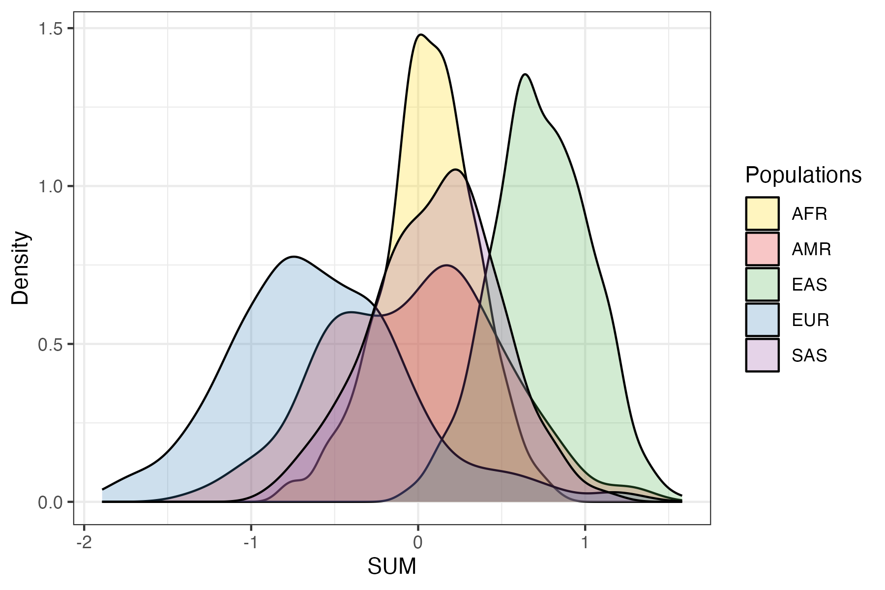
Figure 1. Example of a PGS with shifted distributions in different ancestry groups. Shown here is the distribution of PGS000018 (metaGRS_CAD) calculated using the SUM method in the 1000 Genomes reference panel[1], stratified by genetic ancestry groups (superpopulation labels).

It is important to note that differences in the means between different ancestry groups do not necessarily correspond to differences in the risk (e.g., changes in disease prevalence, or mean biomarker values) between the populations. Instead, these differences are caused by changes in allele frequencies and linkage disequilibrium (LD) patterns between ancestry groups. This illustrates that genetic ancestry is important for determining relative risk, and multiple methods to adjust for these differences have been implemented within the pgsc_calc pipeline.

Note

The pgsc_calc pipeline uses the 1000 Genomes resource[1] as a population reference panel, and uses global ancestry labels (superpopulation) for visualizing PGS distributions and reporting PGS using reference distributions. The panel and the labels are not comprehensive or deterministic, thus we only describe samples from the target dataset in terms of their genetic similarity to these reference populations so as not to transfer labels that may not reflect the new individuals as per recent guidelines.[2]

Methods for reporting and adjusting PGS in the context of ancestry

When a PGS is being applied to a genetically homogenous population (e.g. cluster of individuals of similar genetic ancestry), then the standard method is to normalize the calculated PGS using the sample mean and standard deviation. This can be performed by running pgsc_calc and taking the Z-score of the PGS SUM. However, if you wish to adjust the PGS in order to remove the effects of genetic ancestry on score distributions than the --run_ancestry method can combine your PGS with a reference panel of individuals (default 1000 Genomes) and apply standard methods for adjusting PGS (Figure 2). These methods both start by creating a PCA of the reference panel, and projecting individual(s) into the genetic ancestry space to determine their placement and most similar population. The two groups of methods (empirical and continuous PCA-based) use these data and the calculated PGS to report the PGS.

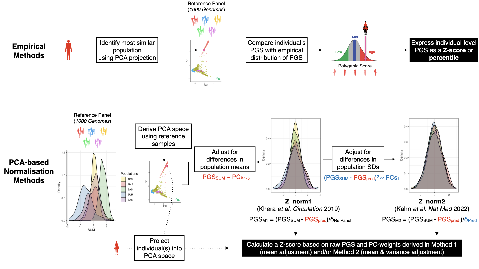
Figure 2. Schematic figure detailing empirical and PCA-based methods for contextualizing or adjusting PGS with genetic ancestry. Data is for the normalization of PGS000018 (metaGRS_CAD) in 1000 Genomes, when applying pgsc_calc --run_ancestry to data from the Human Genome Diversity Project (HGDP) data.

Empirical methods

A common way to report the relative PGS for an individual is by comparing their score with a distribution of scores from genetically similar individuals (similar to taking a Z-score within a genetically homogenous population above).[5] To define the correct reference distribution of PGS for an individual we first train a classifier to predict the population labels (pre-defined ancestry groups from the reference panel) using PCA loadings in the reference panel. This classifier is then applied to individuals in the target dataset to identify the population they are most similar to in genetic ancestry space. The relative PGS for each individual is calculated by comparing the calculated PGS to the distribution of PGS in the most similar population in the reference panel and reporting it as a percentile (output column: percentile_MostSimilarPop) or as a Z-score (output column: Z_MostSimilarPop).

PCA-based methods

Another way to remove the effects of genetic ancestry on PGS distributions is to treat ancestry as a continuum (represented by loadings in PCA-space) and use regression to adjust for shifts therein. Using regression has the benefit of not assigning individuals to specific ancestry groups, which may be particularly problematic for empirical methods when an individual has an ancestry that is not represented within the reference panel. This method was first proposed by Khera et al. (2019)[6] and uses the PCA loadings to adjust for differences in the means of PGS distributions across ancestries by fitting a regression of PGS values based on PCA-loadings of individuals of the reference panel. To calculate the normalized PGS the predicted PGS based on the PCA-loadings is subtracted from the PGS and normalized by the standard deviation in the reference population to achieve PGS distributions that are centred at 0 for each genetic ancestry group (output column: Z_norm1), while not relying on any population labels during model fitting (see Figure 3).

The first method (Z_norm1) has the result of normalizing the first moment of the PGS distribution (mean); however, the second moment of the PGS distribution (variance) can also differ between ancestry groups. A second regression of the PCA-loadings on the squared residuals (difference of the PGS and the predicted PGS) can be fitted to estimate a predicted standard deviation based on genetic ancestry, as was proposed by Khan et al. (2022)[7] and implemented within the eMERGE GIRA.[8] The predicted standard deviation (distance from the mean PGS based on ancestry) is used to normalize the residual PGS and get a new estimate of relative risk (output column: Z_norm2) where the variance of the PGS distribution is more equal across ancestry groups and approximately 1 (see Figure 3).

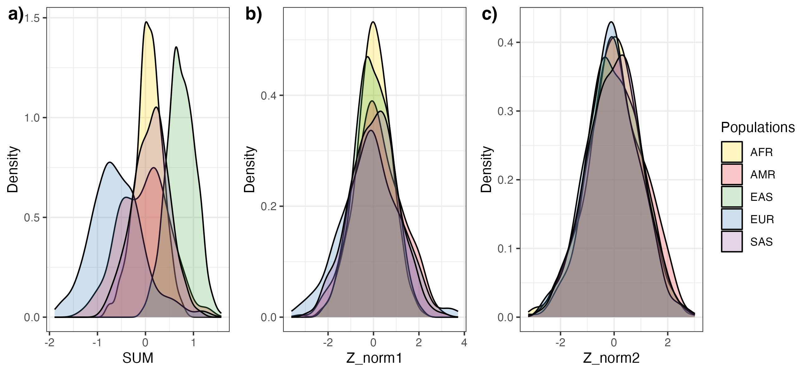
Figure 3. Visualization of PGS distributions before and after PCA-based adjustment. The distribution for the PGS SUM (A) is shown for PGS000018 (metaGRS_CAD) in the 1000 Genomes reference panel, stratified by genetic ancestry groups (superpopulation labels). PCA-based adjustment for differences in the mean (B, Z_norm1) and variances (C, Z_norm2) make the distributions more similar across population labels.

Implementation of ancestry steps within pgsc_calc

The ancestry methods are implemented within the --run_ancestry method of the pipeline (see How do I normalise calculated scores across different genetic ancestry groups? for a how-to guide), and has the following steps:

1. Reference panel: preparing and/or extracting data of the reference panel for use in the pipeline (see How do I set up the reference database? for details about downloading the existing reference [1000 Genomes] [1] or setting up your own).

2. Variant overlap: Identifying variants that are present in both the target genotypes and the reference panel. Uses the INTERSECT_VARIANTS module.

3. PGS Calculation:

   1. Preparing scoring files: in order to normalize the PGS the score has to be calculated on identical variant sets both datasets. The list of overlapping variants between the reference and target datasets are supplied to the MATCH_COMBINE module to exclude scoring file variants that are matched only in the target genotypes.

   2. PGS Scoring: those scoring files are then supplied to the PLINK2_SCORE module, along with allele frequency information from the reference panel to ensure consistent scoring of the PGS SUMs across datasets. The scoring is made efficient by scoring all PGS in parallel.

4. PCA of the reference panel

   1. Preparing reference panel for PCA: the reference panel is filtered to unrelated samples with standard filters for variant-level QC (SNPs in Hardy–Weinberg equilibrium [p > 1e-04] that are bi-allelic and non-ambiguous, with low missingness [<10%], and minor allele frequency [MAF > 5%]) and sample-quality (missingness <10%). LD-pruning is then applied to the variants and sample passing these checks (r² threshold = 0.05), excluding complex regions with high LD (e.g. MHC). These methods are implemented in the FILTER_VARIANTS module.

   2. PCA: the LD-pruned variants of the unrelated samples passing QC are then used to define the PCA space of the reference panel (default: 10 PCs) using FRAPOSA (Fast and Robust Ancestry Prediction by using Online singular value decomposition and Shrinkage Adjustment).[9] This is implemented in the FRAPOSA_PCA module. Note: it is important to inspect the PCA in the report to make sure that it looks correct and places the different reference populations correctly.

5. Projecting target samples into the reference PCA space: the PCA of the reference panel (variant-PC loadings, and reference sample projections) are then used to determine the placement of the target samples in the PCA space using projection. Naive projection (using loadings) is prone to shrinkage which biases the projection of individuals towards the null of an existing space, which would introduce errors into PCA-loading based adjustments of PGS. For less biased projection of individuals into the reference panel PCA space we use the online augmentation, decomposition and Procrustes (OADP) method of the FRAPOSA package.[9] We chose to implement PCA-based projection over derivation of the PCA space on a merged target and reference dataset to ensure that the composition of the target doesn’t impact the structure of the PCA. This is implemented in the FRAPOSA_OADP module. Note: the quality of the projection should be visually assessed in the report - we plan to furhter optimize the QC in this step in future versions.

6. Ancestry analysis: the calculated PGS (SUM), reference panel PCA, and target sample projection into the PCA space are supplied to a script that performs the analyses needed to adjust the PGS for genetic ancestry. This functionality is implemented within the ANCESTRY_ANALYSIS module and tool of our pgscatalog_utils package, and includes:

   1. Genetic similarity analysis: first each individual in the target sample is compared to the reference panel to determine the population that they are most genetically similar to. By default this is done by fitting a RandomForest classifier to predict reference panel population assignments using the PCA-loadings (default: 10 PCs) and then applying the classifier to the target samples to identify the most genetically similar population in the reference panel (e.g. highest-probability). Alternatively, the Mahalanobis distance between each individual and each reference population can be calculated and used to identify the most similar reference population (minimum distance). The probability of membership for each reference population and most similar population assignments are recorded and output for all methods.

   2. PGS adjustment: the results of the genetic similarity analysis are combined with the PCA-loadings and calculated PGS to perform the adjustment methods described in the previous section. To perform the empirical adjusments (percentile_MostSimilarPop, Z_MostSimilarPop) the PGS and the population labels are used. To perform the PCA-based adjusments (Z_norm1, Z_norm2) only the PGS and PCA-loadings are used.

7. Reporting & Outputs: the final results are output to txt files for further analysis, and an HTML report with visualizations of the PCA data and PGS distributions (see pgsc_calc Outputs & report for additional details). It is important to inspect the PCA projections and post-adjustment distributions of PGS before using these data in any downstream analysis.

Citations

[1] (1,2,3)

The 1000 Genomes Project Consortium. (2015) A global reference for human genetic variation. Nature 526:68-74. https://doi.org/10.1038/nature15393.

[2]

National Academies of Sciences, Engineering, and Medicine. (2023) Using Population Descriptors in Genetics and Genomics Research: A New Framework for an Evolving Field. Washington, DC: The National Academies Press. https://doi.org/10.17226/26902

[3]

Reisberg S., et al. (2017) Comparing distributions of polygenic risk scores of type 2 diabetes and coronary heart disease within different populations. PLoS ONE 12(7):e0179238. https://doi.org/10.1371/journal.pone.0179238

[4]

Martin, A.R., et al. (2017) Human Demographic History Impacts Genetic Risk Prediction across Diverse Populations. The American Journal of Human Genetics 100(4):635-649. https://doi.org/10.1016/j.ajhg.2017.03.004

[5]

Folkersen, L., et al. (2020) Impute.me: An Open-Source, Non-profit Tool for Using Data From Direct-to-Consumer Genetic Testing to Calculate and Interpret Polygenic Risk Scores. Frontiers in Genetics 11:578. https://doi.org/10.3389/fgene.2020.00578

[6]

Khera A.V., et al. (2019) Whole-Genome Sequencing to Characterize Monogenic and Polygenic Contributions in Patients Hospitalized With Early-Onset Myocardial Infarction. Circulation 139:1593–1602. https://doi.org/10.1161/CIRCULATIONAHA.118.035658

[7]

Khan, A., et al. (2022) Genome-wide polygenic score to predict chronic kidney disease across ancestries. Nature Medicine 28:1412–1420. https://doi.org/10.1038/s41591-022-01869-1

[8]

Linder, J.E., et al. (2023) Returning integrated genomic risk and clinical recommendations: The eMERGE study. Genetics in Medicine 25(4):100006. https://doi.org/10.1016/j.gim.2023.100006.

[9] (1,2)

Zhang, D., et al. (2020) Fast and robust ancestry prediction using principal component analysis. Bioinformatics 36(11):3439–3446. https://doi.org/10.1093/bioinformatics/btaa152